Execution of Temporal Queries on Third-Party Data
Developing financial software interacting with multiple financial partners quickly becomes a data-intensive exercise in the management of multiple third-party sources of truth, each of which exposing a diverse set of data querying capabilities.
In this article, we discuss the concept of temporal queries, how their execution becomes complex in light of the aforementioned context, and strategies we can adopt to execute sophisticated temporal query patterns on sources with limited capabilities.
What are temporal queries
We define temporal queries as queries involving a point-in-time parameter, asking the underlying system to produce a result based on an internal state cut-off as-of a specified concrete date and time. That is, as opposed to just being able to query a system for its current state, temporal queries give us capabilities to explore the system’s data in time.
We will here be tasking ourselves with the development of a temporal query execution layer, able to process queries on financial data sources that don’t natively support them.
Before diving further: we will anchor our model to an example which we’ll re-use throughout this piece, with the fetching of an account balance at a specific point-in-time on a financial institution through its programmatic interface.
Data sources limitations
One might ask at this point: how come this sort of historical querying capability isn’t a given and natively provided by financial institutions? The answer to this question is beyond the scope of this article and will be left as an exercise to the reader, but involves several factors—ranging from the fact that Financial Institutions is neither a trademark nor a unified body of actors, to the engineering cost of such real-time interfaces when one can instead get away with the provisioning of a PDF report delivered through an FTP directory.
As a result, our main problem here will be to produce reliable values, ensuring that the produced results accurately reflect what they would have been if queried at the specified point-in-time on an otherwise natively capable interface at the source.
Other limitations at the source can exist and will have to be considered in the design of our solution, such as limited querying throughput and interface availability.
Values through time
We’ll need another element of formalism before we can develop our model, and define a value as an atomic, uniquely identified, element of information existing in a particular state.
Constructing off our account illustration, the account balance would be an example of such value, uniquely queryable through the institution interface. This value state would then be defined as the current monetary amount held by the account.
It becomes evident that this state is set up for change. As the account transacts, receiving and spending funds, its balance will transition between different states over time.
Correctness model
As we develop our querying layer, we will want to frame the result it produces in an explicit correctness model, categorizing their accuracy along two dimensions: correctness, and confidence.
| Confidence | Correctness | Result Grade |
|---|---|---|
| Confidently | Correct | A |
| Possibly | Correct | B |
| Confidently | Incorrect | C |
Achieving precision grading of the results will mandate an in-depth understanding of the underlying source value state transitions mechanism, which we explore in the following implementation section.
Query layer architecture
With the above formalism laid out, we can now explore implementation strategies and solutions candidates. We’ll propose the following architecture.
Replicated data layer
In order to support our point-in-time queries, we will create an internal data layer that can overcome the limitations of the underlying sources. We will want this data layer to be kept in sync with the source, supported by mechanisms we’ll describe below, and structured in a way that helps us grade our queries results according to the correctness model we’ve previously defined.
We’ll also consider different data layer designs, with the goal of producing as much grade A results as possible.
The underlying storage technology and specific database used will be kept out of the scope of this article.
Observing values
The simplest implementation of a mechanism we can get away with in order to populate our internal data layer is values observation, which we define by the simple following sequence:
Loop
    1. Query the source for value at time T
    2. Save the source response as a (T, value state) tuple in our layer
End
This approach comes with the advantage of its simplicity. As value states acquired this way are truthful by definition, we get to populate our layer with accurate values through time, at the resolution of our polling interval.
This simplicity of design alas comes with a cost, taking the form of the sub-optimal results grades we can produce.
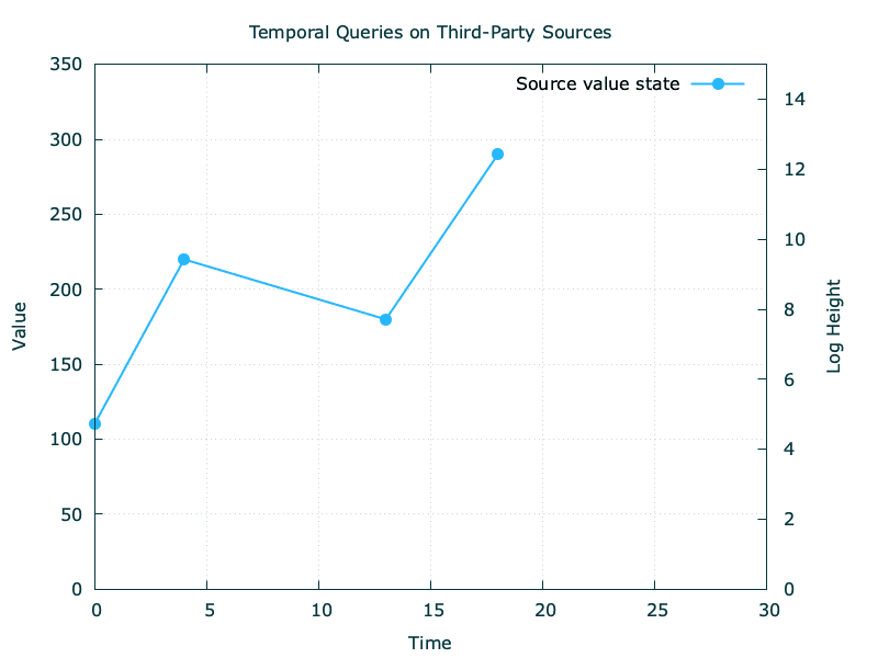
Let’s consider the above values from source and assume an observation every 10 units of time.
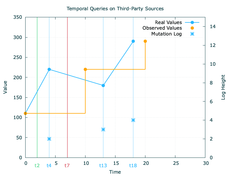
The first problem we’ll encounter is the non-correlation with our observation interval and the likeliness of a value mutation at source, which we highlight here with the real values line: while we observed the value at (t0, t10, t20), the source had changed the value state at (t4, t13, t18).
The reads we’ll operate on our data layer will subsequently be conditioned as follows:
| Confidence | Correctness | Result | Grade |
|---|---|---|---|
| Reads exactly at an observation time | Correct | Confidently Correct | A |
| Reads between two observations | Unknown | Possibly Correct | B |
Without further insights into the likeliness of a mutation, this data layer population mechanism essentially restricts our capability to produce grade A results to reads executed exactly at the time of an observation. While this rhymes with progress and is better than no temporal queries at all, any reads conducted between observations are subject to uncertainty and thus downgraded to grade B, with no possibility of producing grade C results without acquiring more informations from our source.
Mutations logs
We made the case for the need to expand our insight into the specifics of how a source value transitions between states. In this light, we introduce here the abstract concept of a value mutation log, defined as a trail of mutations determining the end state of a value.
Going back to our account balance example, this trail of change would be the list of financial transactions in which this account is finding itself involved.
Log structure
While the source internal implementation specifics remains, well, internal, and thus hidden from our sight, we can devise a set of general attributes to describe mutation logs:
| Attribute | Description | Values |
|---|---|---|
| Availability | Is the log exposed by source at all? | Available, not available |
| Completeness | Is the exposed log exhaustive? | Complete, incomplete |
| Derivativity | Could one derive value states from the log? | Derivative, opaque |
Leveraging the log
With a formal log description framework now set, we can now start to improve our query results by leveraging the source mutation log, assuming it is available.
Constructing off our previous observation mechanism, we will want to derive a first information in the mutation by sourcing the value mutation timestamps from it.
With this additional part of the picture, we can now make our internal data layer aware of the incorrect values it produces based on a proof of obsolescence. This is exemplified below with a read at t7: as we have now proof that the value transitioned to a new state at t4, we can now grade our result as confidently incorrect.
What is interesting to note from the above is that out of the three log attributes we’ve defined, we only needed the log to be available to improve our results grading.
But how do we get to produce confidently correct results? Getting there will require an additional piece information from the mutation log.
Let’s consider the read at t2 illustrated above. From our holistic point of view, we can devise that the result produced will be correct as no value mutation happened between [t0, t4]. From the internals of our data layer, we’ll be in a position to devise so if the log at our disposal is both available and complete, as we’ll need the certitude that no state transition happened. Equipped with this, we can now produce confidently correct results.
We are now in a position to improve the grading of our results:
| Read Time | Result | Grade | Condition |
|---|---|---|---|
| Reads exactly at an observation time | Confidently correct | A | None |
| Reads between two observations | Possibly correct | B | If we don’t know whether we are up to date with the log |
| Confidently correct | A | If we have the certitude that there are no changes in the log | |
| Confidently incorrect | C | If we know there are changes in the log |
Deriving value states
Our journey in the architecture of our execution engine doesn’t stop here though. Assuming we get our hand on an available and complete log, we are positioned to produce grade A and C results and avoid grade B results entirely.
But wouldn’t it be nice to produce only grade A results? Getting there will require us to leverage the last log attribute we’ve defined, derivativity.
We had relied so far on our observations and some second-order data from the mutation log. Going further and using the log content itself gives us the opportunity to complete our observations sequence with re-constructed intermediary states.
Considering that an example log entry could look like the one below:
t4: +110We would be in the position of producing a re-constructed value subsequent to t4 based on our last t0 observation:
t4: 110 (observation at t0) & +110 t4: 220Applying this strategy would let us revise our grade B results and turn them into grade A results, given that we have access to a value log that is both available, complete, and derivative.
Semi-temporal sources
Despite limitations at the querying interface, some sources do happen to be temporally-capable in the realm of their internal system. This leads us to situations where, despite not being able to temporally query the data at source, our model becomes vulnerable to bi-temporal writes at the source.
As an example, consider our previous account balance chart, mapping the values at source to our layer. If the source decides to append at t20 a transaction effective at t7, every value after t7 will be updated at source according to the back-dated mutation—invalidating our initial observations in the process.
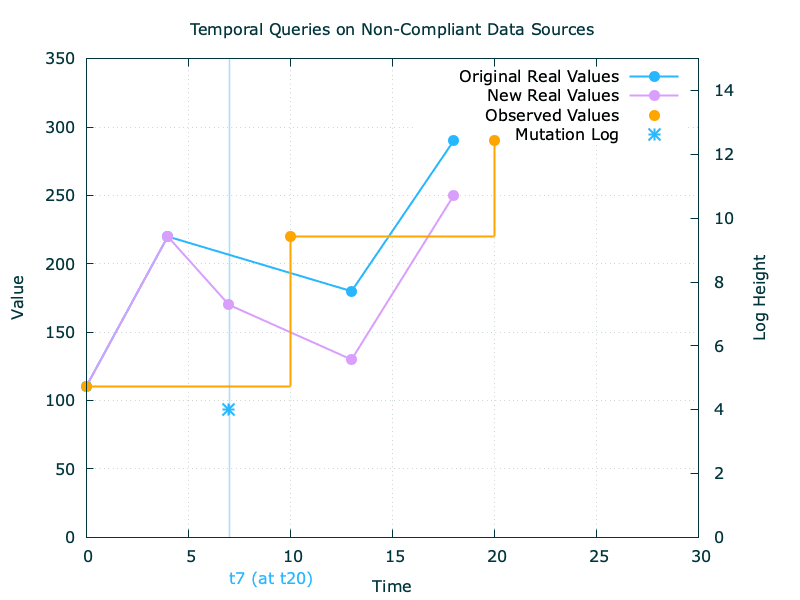
Mitigation strategies will therefore have to invalidate the observation sequence post the effective timestamp of the back-dated log entry, and re-compute their new state to the extent that the log is complete and derivative. Non derivative logs here will lead us to a worst-case situation, where whole frames of multiple observations would then become confidently incorrect.
Conclusion
In our exploration of executing temporal queries on third-party financial data, we've established the need for an internal data layer and different strategies to populate it. These strategies come with different implementation costs and will produce different results grade, which can be summarized as below:
| Primary data | Log Usage | Description | Results |
|---|---|---|---|
| Observations | None | Regularly querying the source for values | Sparse grade A, mostly grade B |
| Observations | Second-order data | Using logs to identify state changes | Grade A and C |
| Observations | Detailed entries data | Reconstructing states using detailed log data | Grade A |